Designed For
Optimizing the Recurring Revenue Model
How to identify signals to deliver above baseline performance.
Establishing Revenue Return Ratios
For every $1 invested in a cohort, these ratios show how many dollars of revenue have come back at 1, 3, 12 and 60 months. The business sets what counts as invested: advertising only, advertising and cost of goods sold, or advertising, cost of goods sold and operating expenses. The return ratios to aim for follow from that choice.
- Month 1
The first read: is the cohort paying, at the rate the plan assumed?
- Month 3
The early shape: are the first upsells or losses showing?
- Month 12
The first year: has the $1 come back, and how fast is the cohort still adding?
- Month 60
The long run: what each $1 becomes over the life of the book.
Each checkpoint matters, and the rate of change between them shows where revenue is improving and what to forecast.
Connecting your investment in people, processes, leads and advertising to revenue takes constant optimization. ABPRO_ lets your team double down on what’s working and cut what’s not.
Revenue
The R2m view from Reporting: each approval cohort’s investment, and the revenue it has returned per $1
The same cohorts as Reporting › Timeline › Revenue › R2m. The lines spread the cohorts apart so each trajectory can be read.
Software-as-a-Service
Subscriptions, cohorts and payback. The billing record is the statement, one row per customer per month, so subscription revenue gets the same cohorts, churn and attribution, tied to the spend that produced it.
- Revenue by signup cohort, followed from the first invoice, with each month attributed back to the cohorts that produced it
- Churn by cohort, split by plan, source, campaign or rep
- Spend to paid: cost per lead, demo and sale, with conversion between every stage
- Payback: dollars returned per $1 at 1, 3, 12 and 60 months, against baseline
- Forecast and concentration: every cohort projected over budget, and how much the top accounts hold
Inputs: the billing export, CRM stages with dates, ad spend by channel and day, commission and team cost, and budgets.
Payments-as-a-Service
Merchant-services ISOs, processors and PayFacs. The recurring revenue is the residual on every merchant’s statement, and ABPRO_ was built on that data, with every MID mapped to the rep and ISO that brought it in.
- Net revenue by statement month, with processing volume and take rate
- Retention and churn rates by cohort, with MIDs new and lost every month
- Every statement month attributed back to its cohorts, reps and ISOs
- Rep and ISO leaderboards and commission on the revenue their merchants produce
- Pricing, card brands and chargebacks, MID by MID, on the same filters as revenue
- Concentration by tier: how much of the book the top merchants hold
Inputs: the summary statement export you already receive, or the processor’s MASS files for line-level detail; CRM stages with dates; ad spend by channel and day; commission and team cost; budgets.
Retention, measured by cohort.
Flagging the merchants at risk is only the start. ABPRO_ measures retention itself: the rates for every cohort, the revenue at stake and where the losses begin, so retention effort is read like any other investment, against baseline.
Retention and churn rates by cohort
Every origination cohort, month by month, by MID count and by revenue, split by rep, ISO, source or pricing.
Revenue potential
What each cohort is on course to produce from its own history: the baseline, what churn takes from it, and what retention adds above it.
Churn traced to where it starts
The reps, ISOs, sources and pricing whose merchants leave early, so retention starts at acquisition.
Retention effort, measured
Each cohort’s actual revenue read against its baseline forecast, so a retention program shows up in dollars every statement cycle.
Power Law Performance
Power Law Performance challenges traditional reporting by intentionally removing the majority of wins, so only above-average results stay in view. What remains is too small a sample to scale on, so we install signals as early in the sales cycle as possible to proxy high-value optimization feedback and maximize our revenue return ratios.
Volume and value run in opposite directions.
Check the book before choosing the metrics. If a minority of accounts make up a large majority of the revenue, the book follows a power law. In these revenue models, optimizing for volume-based metrics (cost per lead, cost per sale, cost per anything) will naturally optimize for lower-value accounts.
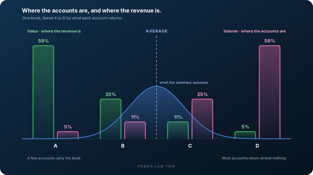
Beat the volume KPI, lower the average.
In 1970 the economist George Akerlof described the mechanism in “The Market for ‘Lemons’”: when buyers can’t tell quality apart at the point of sale, the market prices everything at the average, and the above-average sellers quietly exit.1 His example was used cars. Later work found the same adverse selection in insurance, where buyers know their own risk better than the insurer,2 and in lending, where banks can’t tell safe borrowers from risky ones.3 Michael Spence showed how the better side gets noticed: by sending a signal that is costly to fake.4 Akerlof, Spence and Joseph Stiglitz shared the 2001 Nobel prize in economics for this work.5
That research is about consumer markets and the data buyers and sellers hold about each other. ABPRO_ applies the same mechanism to customer acquisition: judged on volume, an acquisition system can’t see value, so it doesn’t buy any.
Volume-based optimizations are naturally biased against value. Improved performance numbers compound negatively: an expanding market with shrinking margins.
- George A. Akerlof, “The Market for ‘Lemons’: Quality Uncertainty and the Market Mechanism,” Quarterly Journal of Economics 84, no. 3 (1970): 488–500. Journal, Wikipedia.
- Michael Rothschild and Joseph Stiglitz, “Equilibrium in Competitive Insurance Markets: An Essay on the Economics of Imperfect Information,” Quarterly Journal of Economics 90, no. 4 (1976): 629–649. Journal, Wikipedia.
- Joseph E. Stiglitz and Andrew Weiss, “Credit Rationing in Markets with Imperfect Information,” American Economic Review 71, no. 3 (1981): 393–410. JSTOR, Wikipedia.
- Michael Spence, “Job Market Signaling,” Quarterly Journal of Economics 87, no. 3 (1973): 355–374. Journal, Wikipedia.
- The Nobel Prize in Economic Sciences 2001, awarded to George A. Akerlof, A. Michael Spence and Joseph E. Stiglitz “for their analyses of markets with asymmetric information.” nobelprize.org.
Optimizing for Power Law
Label the book, then read it backwards.
Split the book in half on the average, then split each half again: four tiers, A to D. Then trace the tiers back through the funnel to the earliest signal that predicts them.
- 1
Identify Above Avg.
Tier every account from the statements it produces, on the same rule every month, and mark the ones running above the average.
- 2
Apply Attribution
Attribute each tier back to the sources, campaigns, pages and reps that produced it, to find the early traits that lean toward the top tiers.
- 3
Implement Signals
Put those traits to work as early in the funnel as they show up: in targeting, in lead scoring and in routing to sales.
- 4
Optimize
Move spend toward what produces above-baseline accounts, read R2m as it comes in, and repeat every statement cycle.
The earlier in the funnel a signal can be identified and anchored, the bigger its impact on value.
Aim at value, and the revenue target follows.
It sounds backwards. The way to exceed a revenue target isn’t to chase the revenue number harder. Find the early signal, aim marketing at it, route the accounts that can carry the book to sales, and let each team do its job on the right metrics. Results beat the baseline the plan assumed, margins go up, and the target is reached from underneath.
That’s what ABPRO_ is for: reading investment through to revenue and back, every statement cycle, and flagging what runs above and below baseline while there’s still time to move the money.
See the shape of your own book.
Book your demo and we’ll present the platform on a demo portfolio, then review where your revenue comes from.